Question:
A company currently ships products from 5 plants to 4 warehouses. The company is considering the option of closing down one or more plants. This would increase distribution cost but perhaps lower overall cost. The company’s objective is to minimize the total cost. Formulate this as an optimization problem to be able to find out what plants, if any, should the company close, and the number of products to be shipped from each plant to each warehouse.
| Transportation Costs (per product) | |||||
| Plant 1 | Plant 2 | Plant 3 | Plant 4 | Plant 5 | |
| Warehouse 1 | $4 | $2 | $3 | $2.5 | $4.5 |
| Warehouse 2 | $2.5 | $2.6 | $3.4 | $3 | $4 |
| Warehouse 3 | $1.2 | $1.8 | $2.6 | $4.1 | $3 |
| Warehouse 4 | $2.2 | $2.6 | $3.1 | $3.7 | $3.2 |
| Demand | |
| Warehouse 1 | 15 |
| Warehouse 2 | 18 |
| Warehouse 3 | 14 |
| Warehouse 4 | 20 |
| Capacity (x 1000 products) | Fixed costs ($) | |
| Plant 1 | 20 | 12000 |
| Plant 2 | 22 | 15000 |
| Plant 3 | 17 | 17000 |
| Plant 4 | 19 | 13000 |
| Plant 5 | 18 | 16000 |
Answer:
To address this problem, we can start with a simple table where we will put all the values in one place so that it will look accessible.
| From To-> | Warehouse 1 | Warehouse 2 | Warehouse 3 | Warehouse 4 | Supply |
| Plant 1 | 4 | 2.5 | 1.2 | 2.2 | 20 |
| Plant 2 | 2 | 2.6 | 1.8 | 2.6 | 22 |
| Plant 3 | 3 | 3.4 | 2.6 | 3.1 | 17 |
| Plant 4 | 2.5 | 3 | 4.1 | 3.7 | 19 |
| Plant 5 | 4.5 | 4 | 3 | 3.2 | 18 |
| Demand | 15 | 18 | 14 | 20 |
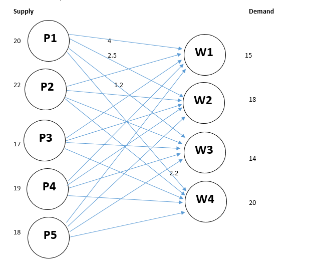
Here 20 number of relation available
XP1W1 = Number of Product shipped from Plant 1 to Warehouse 1
.
.
XP5W4 = Number of Product shipped from Plant 5 to Warehouse 4
XPiWj = Number of Product shipped from Plant i to Warehouse j
Where, i = Plant 1-5, j = Warehouse 1-4
Objective function
Min [12000 + 4 XP1W1 + 2.5 XP1W2 + 1.2 XP1W3 + 2.2 XP1W4 + 15000 + 2 XP2W1 + 2.6 XP2W2 + 1.8 XP2W3 + 2.6 XP2W4 + 17000 + 3 XP3W1 + 3.4 XP3W2 + 2.6 XP3W3 + 3.1 XP3W4 + 13000 + 2.5 XP4W1 + 3 XP4W2 + 4.1 XP4W3 + 3.7 XP4W4 + 16000 + 4.5 XP5W1 + 4 XP5W2 + 3 XP5W3 + 3.2 XP5W4]
Constraints:
Supply Constraints:
XP1W1 + XP1W2 + XP1W3 + XP1W4 ≤ 20
XP2W1 + XP2W2 + XP2W3 + XP2W4 ≤ 22
XP3W1 + XP3W2 +XP3W3 + XP3W4 ≤ 17
XP4W1 + XP3W2 + XP3W3 + XP3W4 ≤ 19
XP4W1 + XP3W2 + XP3W3 + XP3W4 ≤ 18
Total Supply ≤ 96
Demand Constraints
XP1W1 + XP2W1 + XP3W1 + XP4W1 + XP4W1 = 15
XP1W2 + XP2W2 + XP3W2 + XP4W2 + XP5W2 = 14
XP1W3 + XP2W3 + XP3W3 + XP4W3 + XP5W3 = 18
XP1W4 + XP2W4 + XP3W4 + XP4W4 + XP5W4 = 20
XPiWj ≥ 0
Implementation in Excel:
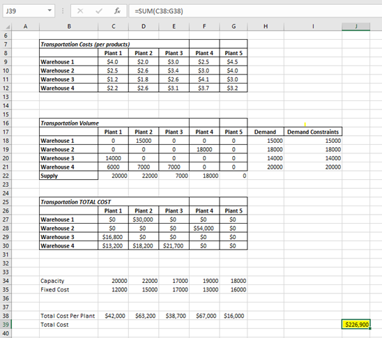
In the first table the Transportation Costs are put as it is given in the question.
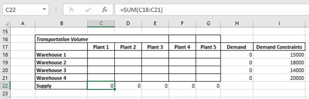
Transportation Volume Table:
But there is some work has been done in the second table (Transportation Volume).
We know in general
Total cost = (production cost + Transportation cost) * quantity + fixed cost
Here production cost is not mentioned hence we can write
Total cost = Transportation cost * quantity + fixed cost
To find out total cost we have transportation cost from plants to warehouse and fixed cost of the plants.
In this question plants in total production capacity is higher than the demand. So to use the plants efficiently as well as to meet the demand we have to find out the optimum plant production as not all the plants are equally efficient in terms of the fixed cost and the transportation cost.
So our goal is to find out the optimum production volume of each plant.
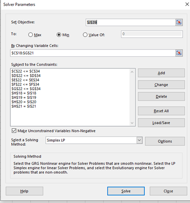
To achieve this goal, we will use Microsoft Excel Solver function.
Demand Constraints:
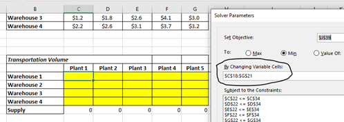
Before using the function, we have to put the constraints into this excel file.
One thing we can take for granted in this question, which is we have to meet the demand, hence we have put the demand in the I column and given a constraint that $H$18 = $I$18 and so on. To make this happen we have to vary the production in the plants as well.
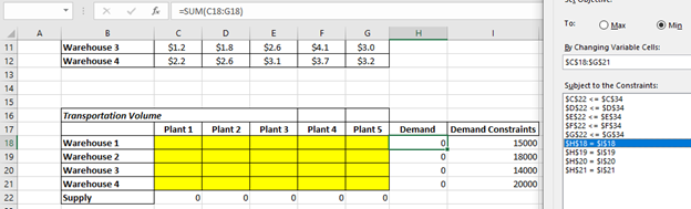
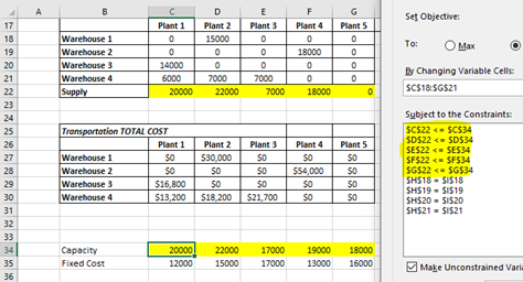
So we made the yellow marked 20 cells as variable cells.
At the end the Demand column will also accumulate the all the plants supply to the warehouses separately (H18 = SUM(C18:G18) and so on) and Supply row will accumulate the different Plants supply quantity to different warehouses (C22 = SUM(C18:C21) and so on)
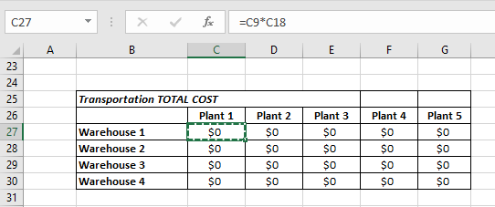
Transportation Total Cost Table:
We will simply multiply transportation cost with product quantity.
Total Cost Per Plant:
Total cost can be calculated by adding the plant production and the fixed cost.
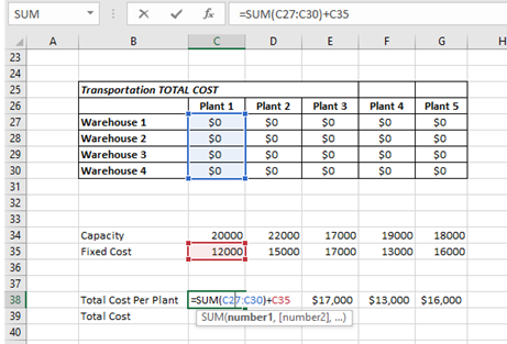
Capacity Constraints :
Each of the plants can produce up to its given capacity, hence the total transported units from each plant is less than or equal to the plant capacity. Capacity constraints can be implement by this way (C22 ≤ C34 and so on)
Objective function:
Objective function is J39 = SUM(C38:G38) to be minimum
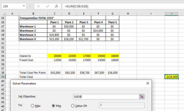
Final Result:
In the second table: Transportation Volume, we can see that the total transported unit from Plant 5 is zero to all warehouse.
Which means for operating cost to be minimum Plant 5 to be shut down.
We can also see that Plant 1 & 2 is operating at its highest capacity and Plant 3 is used lesser than other three plants.